Graph Representation Learning
huyi / July 2022
- chap1 Introduction
- chap2 Background and Traditional Approaches
- chap 3: Neighborhood Reconstruction Methods
- chap 4: Multi-relational Data and Knowledge Graphs
chap1 Introduction
1.1 What is a graph?
$\mathcal{G=(V,E)}$
simple graph,directed graph, directed graph with weighted edges可以由adjacency matrix来表示
simple graph: 其中的边undirected,且没有自己指向自己的节点)
directed graph就是adjacency matrix不对称而已
1.1.1 Multi-relational Graphs
different types of edges extend the edge notation to include an edge or relation type $\tau$ , e.g., $(u, \tau, v)\in\mathcal{E}$,对于每一种type $\tau$ 可以有一个adjacency matrix–>adjacency tensor $\mathcal{A}\in\mathbb{R}^{\mathcal{|V|\times|R|\times|V|}}$, 其中 $\mathcal{R}$是 relations的集合
- Heterogeneous graphs
nodes也有types, 根据这些type可以把nodes分成各不相交的k个集合:
$\mathcal{V=V_1\cup V_2\cup…\cup V_k}$ where $\mathcal{V_i\cup V_j}=\emptyset$
一般来说,一种relation专门连接两种特定的节点,比如$\tau_i$ 专门连接$\mathcal{V_k} and \mathcal{V_j}$
也有可以连接多种节点类型的relation type
-
Multiplex graphs 图可以被分成k layers, each layer corresponds to a unique relation.
Intra-layer edges: 一种专门的edge Inter-layer edges: 看一个节点生出来的不同类型的edges
1.1.2 Feature Information
node-level attributes that we represent using a real-valued matrix: $\mathsf{X}\in\mathbb{R}^{\mathcal{|V|\times m}}$
$\mathcal{|V|}$个节点,每个节点m维向量
注:节点顺序和adjacency matrix里面的节点顺序相同
很少考虑edge在除了types之外还有自己的feature
1.2 Machine learning on graphs
problem-driven
分类不可直接沿用 supervised / unsupervised
图机器学习的任务类型:
1.2.1 Node classification
the goal is to predict the label $y_u$ associated with all the nodes $u \in V$, when we are only given the true labels on a training set of nodes $V_{train}\subset\mathcal{V}$.
node classification和标准的supervised classification 区别:
    nodes in standard supervised classification: independent and identically distributed
    nodes in graph machine learning: interconnected-->model the relationships between nodes
由于我们可以接触到test nodes的一些信息,所以不完全算unsupervised–>semi-supervised
1.2.2 Relation prediction
别名:link prediction, graph completion, relational inference
standard setup:有一堆nodes $\mathcal{V}$, 一堆incomplete set of edges $\mathcal{E}$ \ $\mathcal{E}_{train}$
1.2.3 Clustering and community detection
接近于unsupervised
1.2.4 Graph classification, regression, and clustering
chap2 Background and Traditional Approaches
what’s used before the advent of modern deep learning approaches?
针对三种不同的学习任务:
• node and graph classification tasks: basic graph statistics, kernel methods
• relation prediction: various approaches for measuring the overlap between node neighborhoods,
• clustering or community detection on graphs: spectral clustering using graph Laplacians
2.1 Graph Statistics and Kernel Methods
traditional way: extracting some statistics or features—based on heuristic functions or domain knowledge—and then use these features as input to a standard machine learning classifier
–>introduce some important node-level features and statistics
–>how these node-level statistics can be generalized to graph-level statistics
–>extended to design kernel methods over graphs
==>GOAL: introduce various heuristic statistics and graph properties
2.1.1 Node-level statistics and features
以Medicis家族的social network为例:
what properties or statistics of the Medici node distinguish it from the rest of the graph?
what are useful properties and statistics that we can use to characterize the nodes in this graph?
Node degree
$d_u=\sum\limits_{u\in V}\mathsf{A}[u,v]$表示这个节点伸出来的边的个数
Node centrality \(e_u=\frac{1}{\lambda}\sum\limits_{v\in V}\mathsf{A}[u,v]e_v\) 即centrality和neighbour的centrality 的 weighted sum成正比,其中$\lambda$为一个常数,按照上面的公式,可以发现e是Adjacency matrix的本征矢: \(\lambda e=\mathsf{A}e\)
还有其他的centrality:
- betweeness centrality: how often a node lies on the shortest path between two other nodes
- closeness centrality: measures the average shortest path length between a node and all other nodes
The clustering coefficient
- –>structural distinction
–>proportion of closed triangles in a node’s local neighborhood
–>how many pairs of nodes there are in u’s neighborhood

- another way of viewing: ego graph: the subgraph containing that node,, its neighbors, and all the edges between nodes in its neighborhood
2.1.2 Graph-level features and graph kernels
- 先前的讨论都是node-level的,无论是classification problem还是features 和 statistics.
- 那 graph-level classification怎么办? 这一节的大多方法算在graph kernel methods中 graph kernels,Kriege et al. 2020
Bag of nodes simply aggregating nodelevel statistics
The Weisfeiler-Lehman kernel iterative neighborhood aggregation: 通过迭代来包含整个图的信息(neighbour的neighbour的neighbour……)
basic idea:
- assign an initial label $l^{(0)}(v)$ to each node. 通常使用digree这个feature: $l^{(0)}(v)=d_v$
- iteratively assign a new label to each node by hashing the multiset of the current labels within the node’s neighborhood
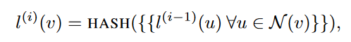 上述公式里面的“”表示multi-set(其中可以有重复的数),HASH表示一种映射:
HASH:$\mathbb{R}^{|\mathcal{N}|}\rightarrow\mathbb{R}$
上述公式里面的“”表示multi-set(其中可以有重复的数),HASH表示一种映射:
HASH:$\mathbb{R}^{|\mathcal{N}|}\rightarrow\mathbb{R}$
- K次迭代后,$l^{(K)}(v)$代表了K-hop neighbourhood –> feature representation for the graph
Graphlets and path-based methods node-level discussion中, 有一种确定graph feature的方法是数某种特征的subgraph的数量, 在此可以叫 graphlet.
the graphlet kernel:
- enumerating all possible graph structures of a particular size
- counting how many times they occur in the full graph
alternative to enumerating:path-based method
只需要关心graph中不同的paths.
比如:the random walk kernel (2003) involves running random walks over the graph and then counting the occurrence of different degree sequences
比如:shortest-path kernel (2005) involves a similar idea but uses only the shortest-paths between nodes (rather than random walks)
? degree sequence是啥
2.2 Neighborhood Overlap Detection
回顾上节:
上节讲node/graph-level features.
上节问题:
这些features并不能quantify the relationships between nodes
上面的features对relation prediction任务就没什么大用
本节关心的:
- neighborhood overlap between pairs of nodes–>关心一对点之间二者的相关性有多强(pair of nodes)
-
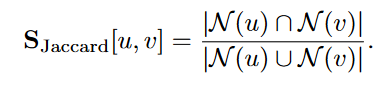
最简单的方法:$\mathsf{S}[u,v]= \mathcal{N}(u)\cap\mathcal{N}(v) $ $\mathsf{S}\in\mathbb{R}^{\mathcal{ V \times V }}$是similarity matrix–>summarizing all the pairwise node statistics -
Adjacency matrix 和 similarity matrix之间的关系
2.2.1 Local overlap measures
-
Sorensen index: 一个$\mathcal{ V \times V }$维的矩阵 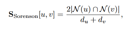
-
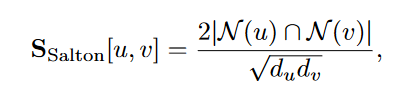
Salton index:
-
Jaccard overlap:
-
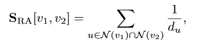
Resource Allocation (RA) index counts the inverse degrees of the common neighbors
-
Adamic-Adar (AA) index performs a similar computation using the inverse logarithm of the degrees
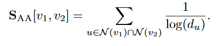
以上两种 index 相当于给了 low-degree neighbour 更高的权重,因为直觉上,a shared low-degree neighbor is more informative than a shared high-degree one.
2.2.2 Global overlap measures
只考虑local overlap(1-hop)不够:two nodes could have no local overlap in their neighborhoods but still be members of the same community in the graph.
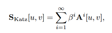
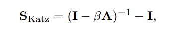
Katz index
 根据下面的理论可以改写成这个形式:
 $\mathsf{A}^i[u,v]$表示了从u到v,i步的path的条数。
如果$\beta<1$,long path的权重就会降低
Geometric series of matrices
> Theorem 1. *Let X be a real-valued square matrix and let λ1 denote the largest eigenvalue of X.*,,则有:

<br>$\mathsf{(I-X)^{-1}}=\sum\limits_{i=0}^{\infin}\mathsf{X^i}$

<br>当且仅当 λ1 < 1 且 (I-X) 满秩。
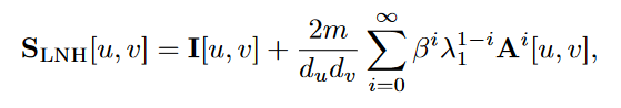
Leicht, Holme, and Newman (LHN) similarity
-
Katz index的问题: strongly biased by node degree, 容易给high-degree nodes更高的similarity score
-
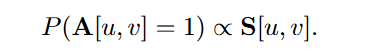
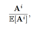
new method: ratio between the actual number of observed paths and the number of expected paths between two nodes
-
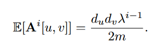
E [ A^i ] 的计算 利用 configuration model assumes that we draw a random graph with the same set of degrees as our given graph. –>
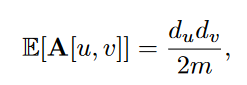
其中m是所有图中一共有多少条边。random configuration model下,两个节点间的edge出现的可能性和两节点各自的度数正相关。
可以这么理解:有d_u条边离开u,每条边有d_v/2m的机会最后到v ? 为什么是d_v/2m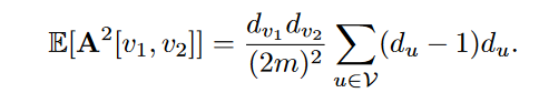
$v_1$–>u–>$v_2$ $\frac{d_{v_1}d_{v_2}}{2m}\cdot\frac{d_{v_2}(d_{u}-1)}{2m}$
-
问题: 3-hop以上就很难算
-
3-hop及以上的问题:
- the largest eigenvalue can be used to approximate the growth in the number of paths.
其中p_i是节点u跟其他节点间长为i的路径条数。
为什么p_i会收敛到eigenvector?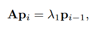
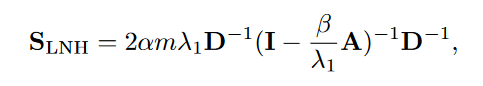
D是表示节点数量的对角阵
-
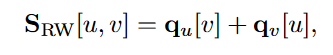
Random walk methods
stochastic matrix $P = AD^{-1}$
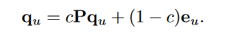
solution:
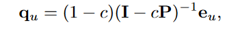
–>
2.3 Graph Laplacians and Spectral Methods
goal: clustering learn low dimensional embeddings of nodes
2.3.1 Graph Laplacians
- 图的邻接矩阵可以表示整个图的信息,但也有其他矩阵可以表示图。
- 这些矩阵叫 Laplacians ,可以通过 adjacency
PART I : Node Embeddings
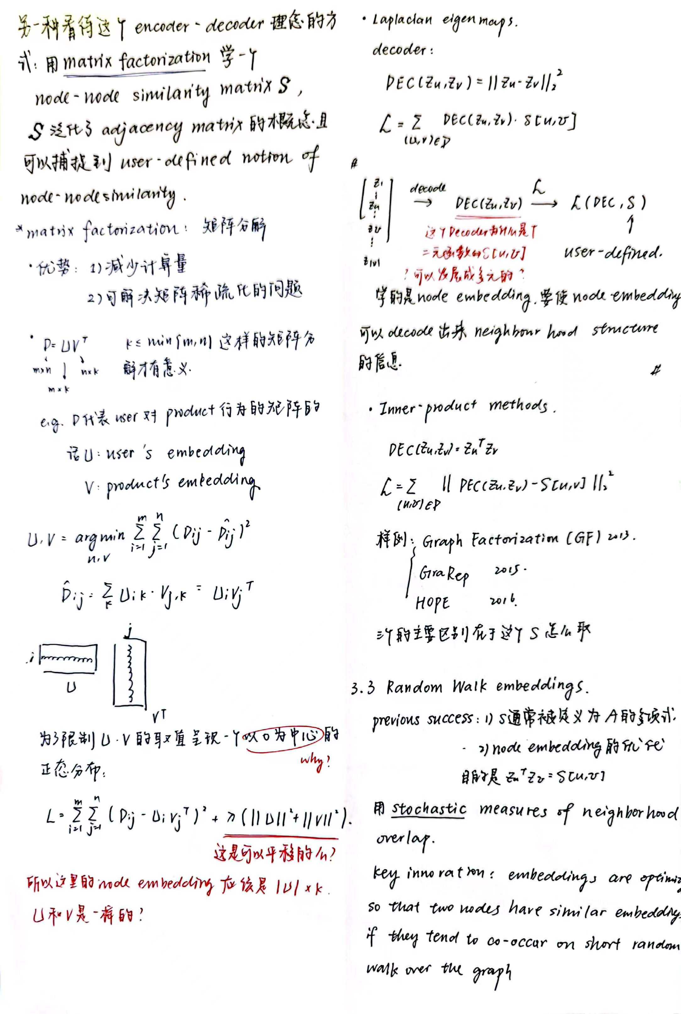
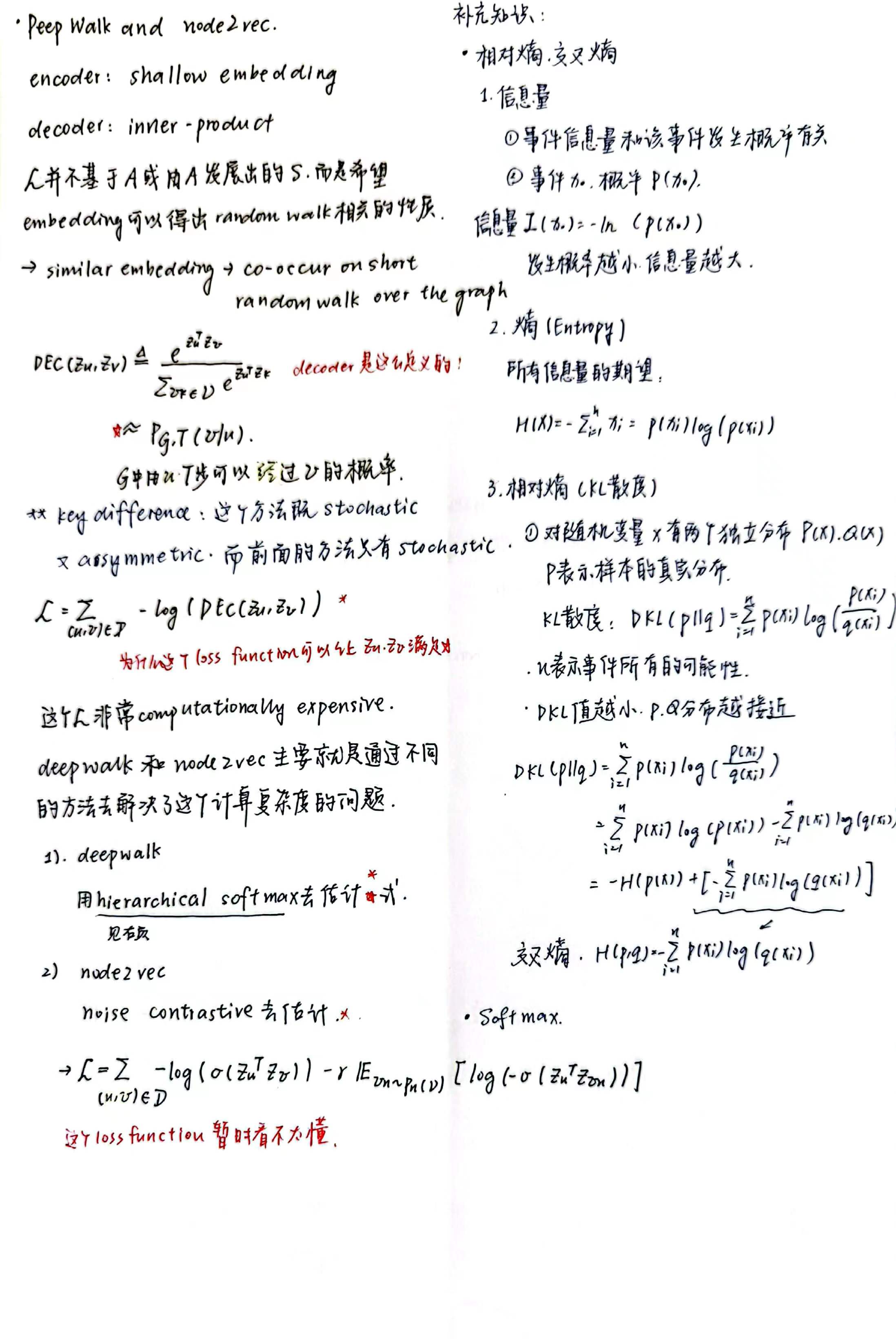
chap 3: Neighborhood Reconstruction Methods
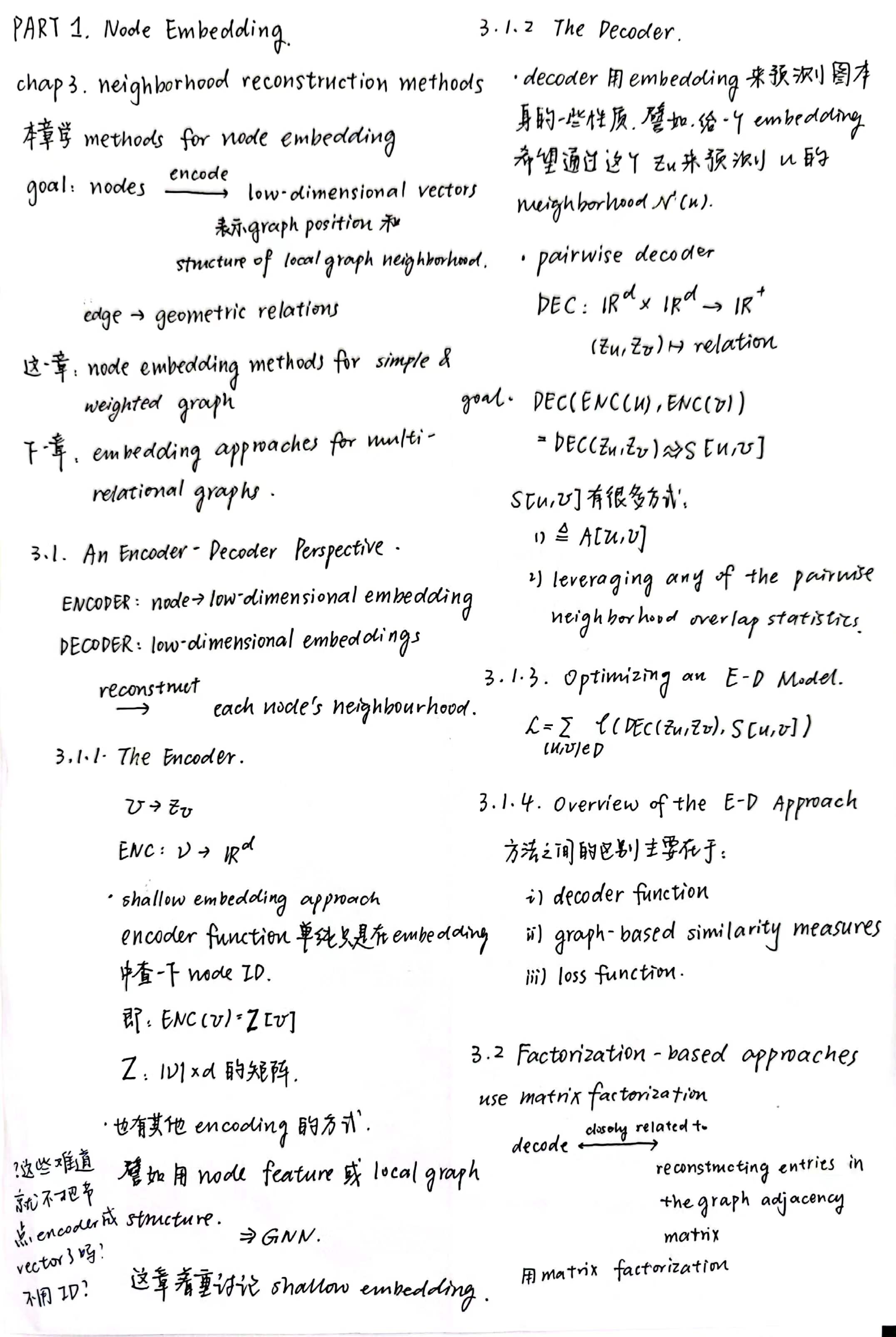
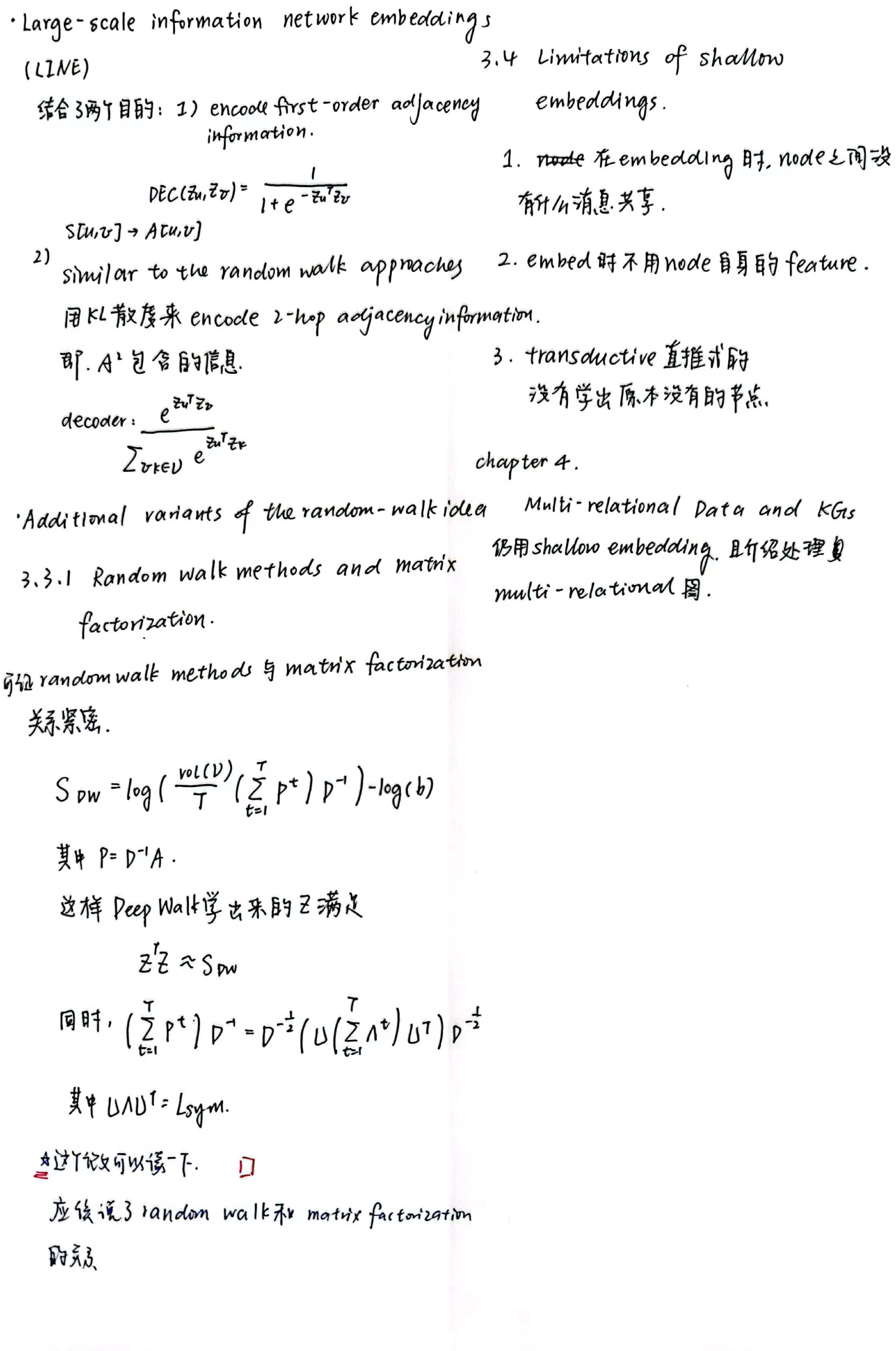
chap 4: Multi-relational Data and Knowledge Graphs
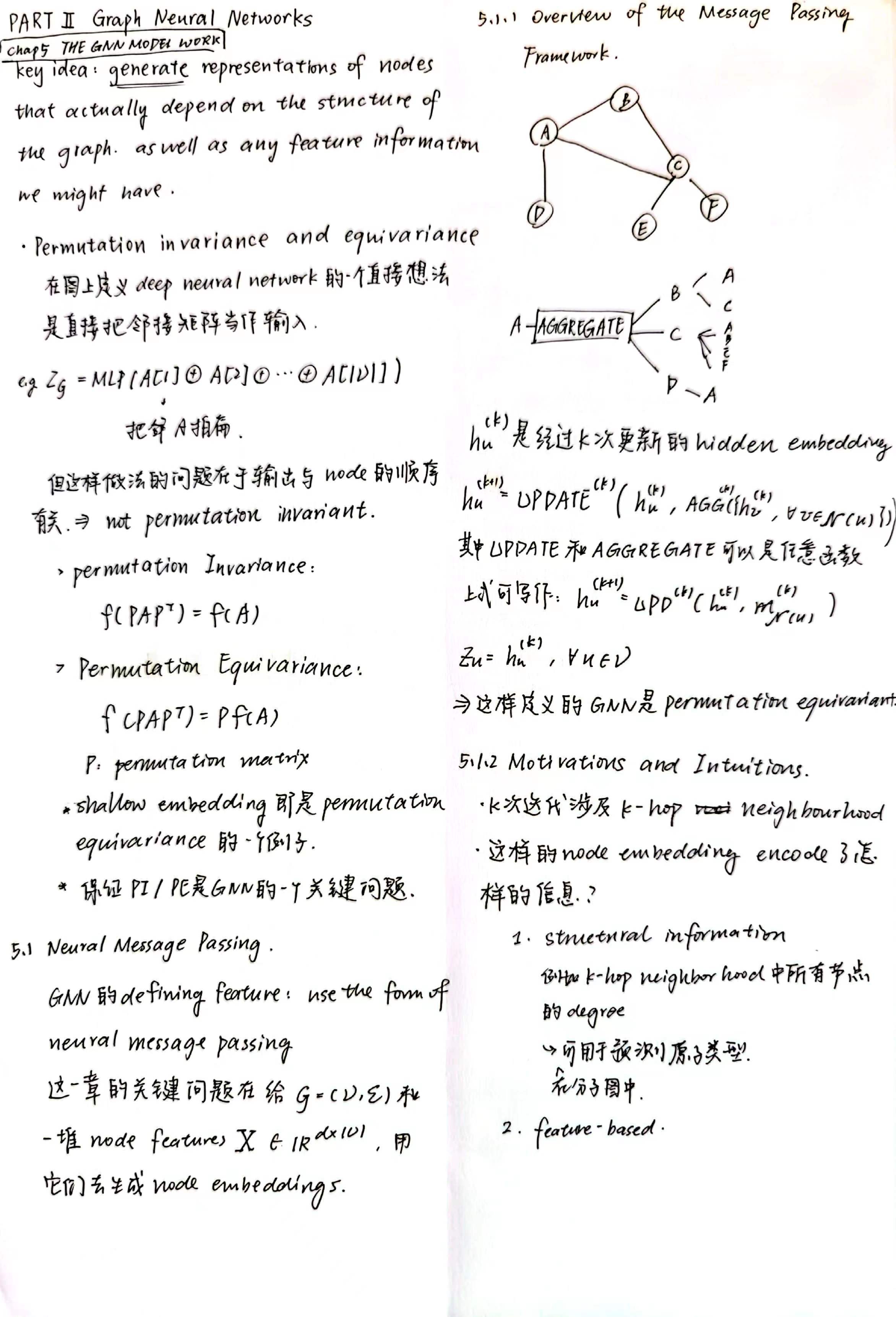
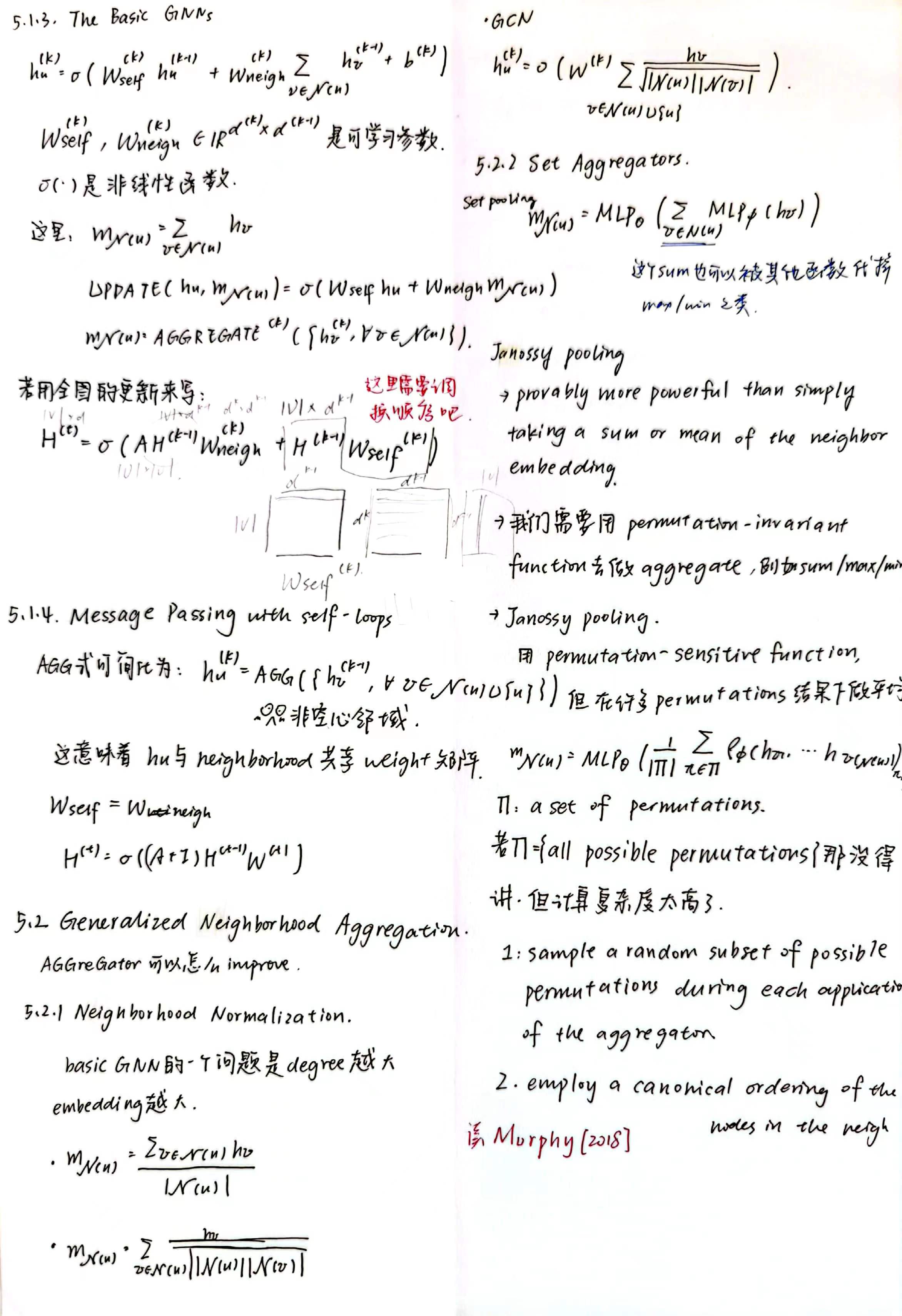
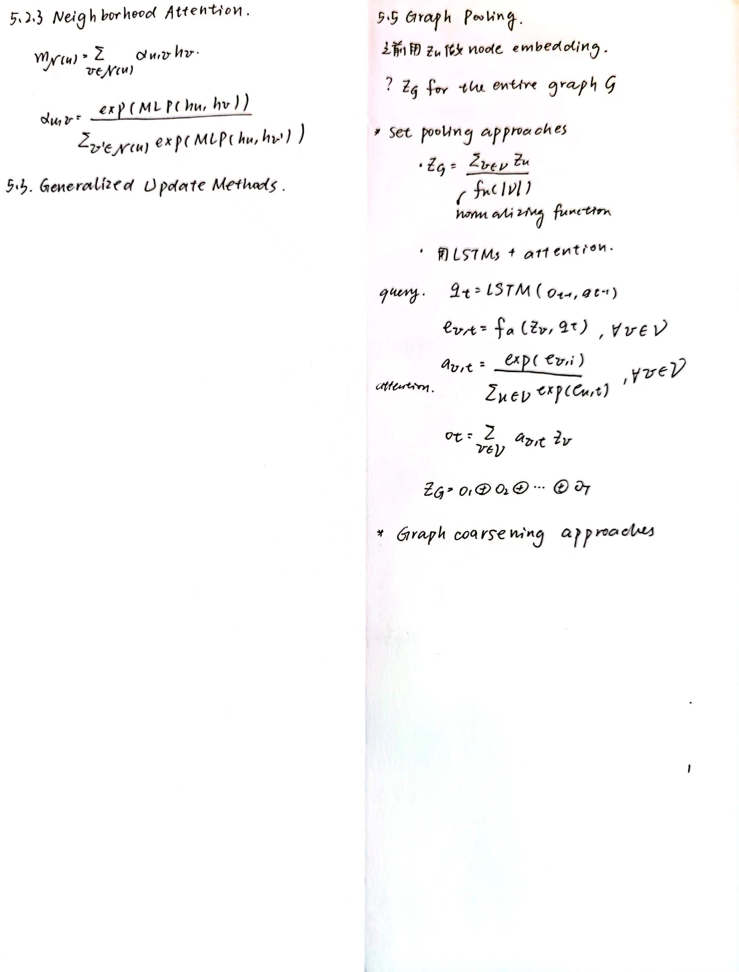
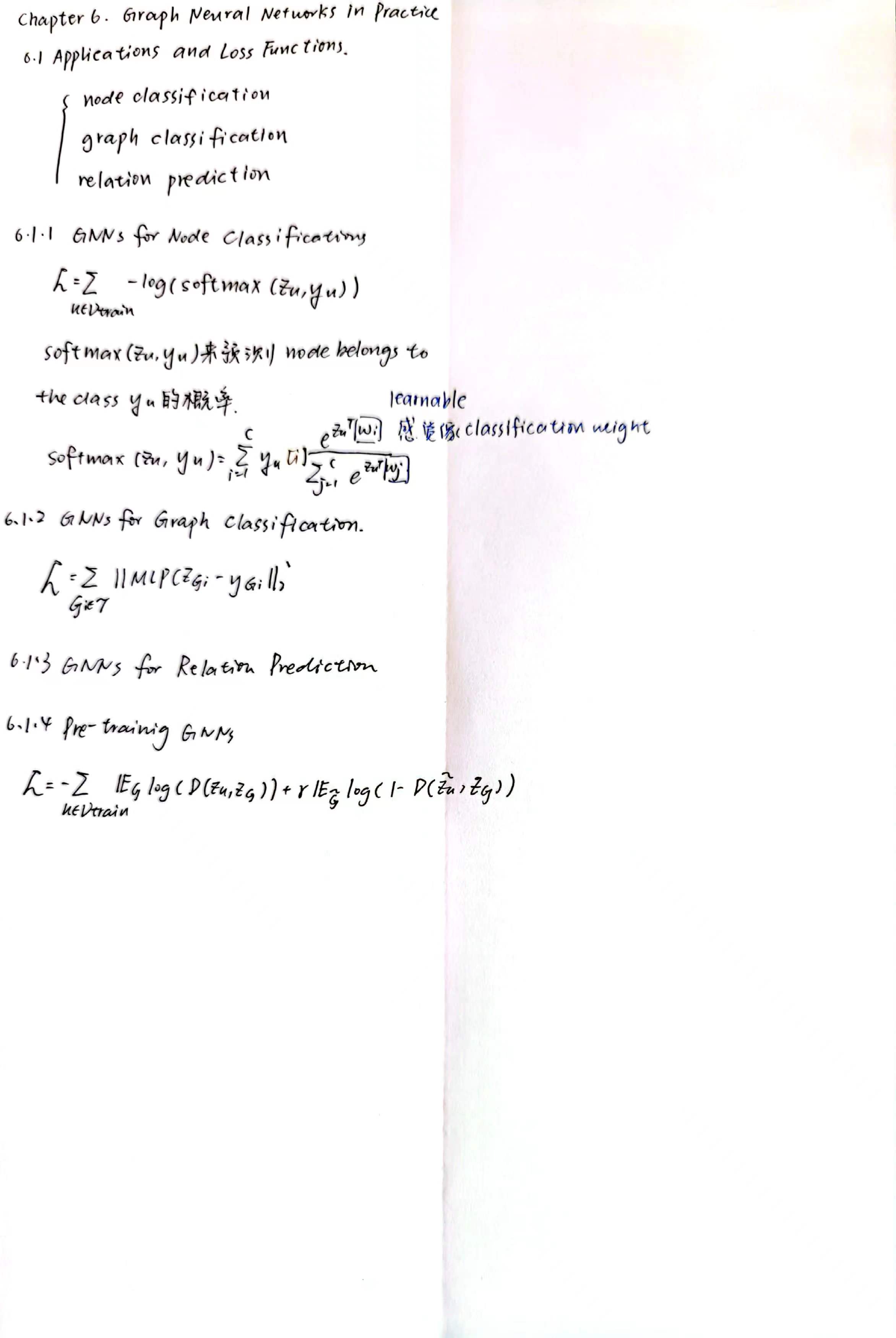
PART II : Graph Neural Network